Build Your Own Inference Engine: From Scratch to "7"

Building a C++ Inference Engine from scratch, part 1

Aug 04, 2024

I like to keep things practical. Let’s train a simple neural network, save the model, and write an inference engine that can execute inputs against the model. Sounds like a fun time to me!

Training a model

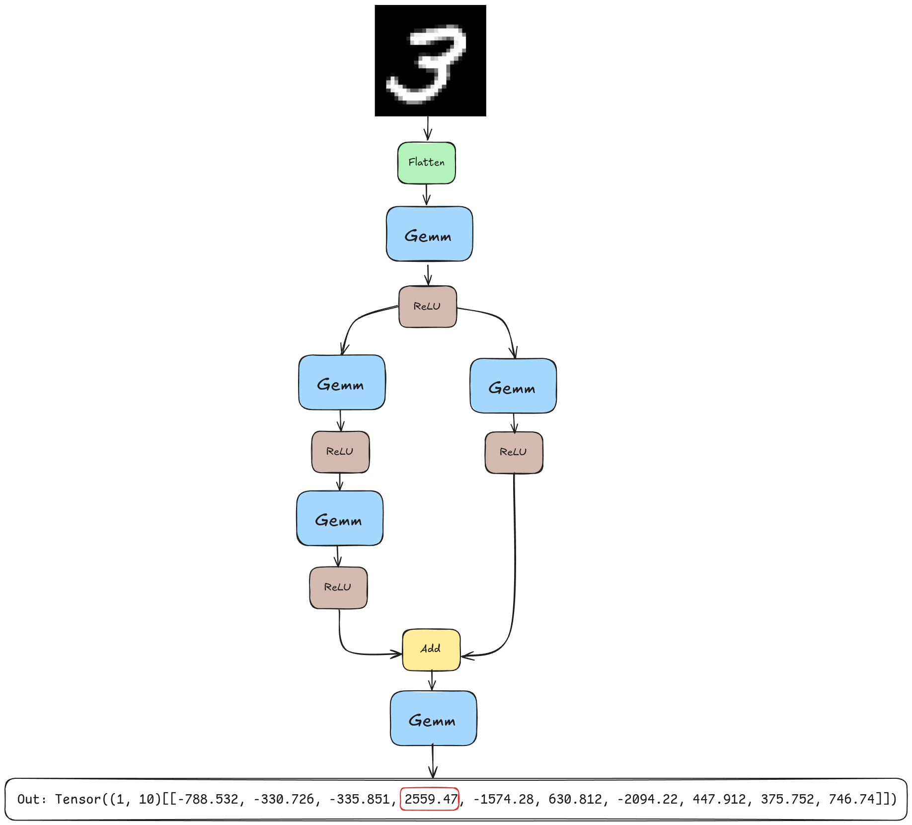
Before we can serve a model, we need to train one. We’ll be using the model illustrated below.

This model has some nice features: it’s easy to train, has a non-trivial topology, and only requires 4 operations: Flatten, Gemm, ReLU, and Add. Gemm stands for generalized matrix multiplication. I think the others are self-explanatory.

We want to save the trained model in ONNX format. ONNX is a standard format for saving models for interoperability between different ML frameworks. Since I probably won’t be adding support for other model formats, this is a solid default choice.

You can see all the code related to training the model on my github.

(venv) michal@michal-lg:~/code/mnist$ python nn_complex.py 
Net(
  (fc1): Linear(in_features=784, out_features=512, bias=True)
  (fc2_left): Linear(in_features=512, out_features=200, bias=True)
  (fc2_left2): Linear(in_features=200, out_features=100, bias=True)
  (fc2_right): Linear(in_features=512, out_features=100, bias=True)
  (fc3): Linear(in_features=100, out_features=10, bias=True)
)
Epoch 1 - Test loss: 0.0006, Accuracy: 84.77%
Epoch 2 - Test loss: 0.0004, Accuracy: 89.66%
Epoch 3 - Test loss: 0.0003, Accuracy: 90.73%
Epoch 4 - Test loss: 0.0003, Accuracy: 91.91%
Epoch 5 - Test loss: 0.0003, Accuracy: 92.58%
Epoch 6 - Test loss: 0.0002, Accuracy: 93.31%
Epoch 7 - Test loss: 0.0002, Accuracy: 93.59%
Epoch 8 - Test loss: 0.0002, Accuracy: 94.02%
Epoch 9 - Test loss: 0.0002, Accuracy: 94.23%
Epoch 10 - Test loss: 0.0002, Accuracy: 94.65%
Model saved as mnist_ffn_complex.onnx

With the model trained, let’s learn more about inference engines.

Why inference engines matter

Before designing the engine, let’s discuss why we even want one in the first place. Couldn’t we just reuse the same ML training framework we used to train the model?

With LLMs going mainstream, an interesting observation was made - over the lifetime of a model, serving can be more expensive than training. So it makes sense to have specialized tools optimized for inference specifically.

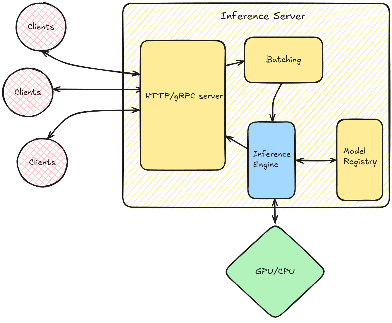
Inference servers are software for managing deployment, lifetime, and serving-related optimizations of already trained models. Popular inference servers include Nvidia’s Triton Inference Server or Google’s TensorFlow Serving.

Inference servers balance throughput and latency. Throughput is often optimized through dynamic batching - waiting for inference requests to accumulate before handing them off to the inference engine. This improves hardware utilization at the cost of increased latency for some requests.

Illustration of an inference engine and its components.

The inference engine, the subject of our discussion, then efficiently executes the model with provided inputs. To achieve high performance, inference engines employ a range of optimizations:

Hardware acceleration
Efficient memory management
Graph optimizations
Quantization to reduce numeric precision while maintaining accuracy

I want to implement graph optimizations and GPU acceleration in follow-up posts. Consider subscribing to get an email when I publish the next post.

For now, let’s stick with CPU inference.

Inference engine from scratch

Let’s outline the steps that our engine will do:

Load the model
Construct a graph representation of the model
Topologically sort nodes
Run inference with user inputs

Loading the model

Luckily for us, ONNX models are saved in Protobuf format. This means we can download the onnx-ml.proto and generate a client library for interacting with ONNX files. This will also be our only external dependency - sticking with just the standard lib from now on.

Once the model is loaded, we can extract the weights into a Tensor object. Tensor is a thin wrapper around std::vector<T> where elements are stored in row-major order.

Graph construction

In this part, we iterate over all nodes in the ONNX model, extract each into a minimal Node representation, and store them in an adjacency list in a Graph object.

Nodes simply define the operation and list the names of input and output tensors.

When we construct the graph, we add nodes 1-by-1. When a new node is added, we check if any existing nodes are the parents or children of the new node by comparing input and output tensor names.

Now that we have a graph, we have to figure out how to execute it.

Topological sorting

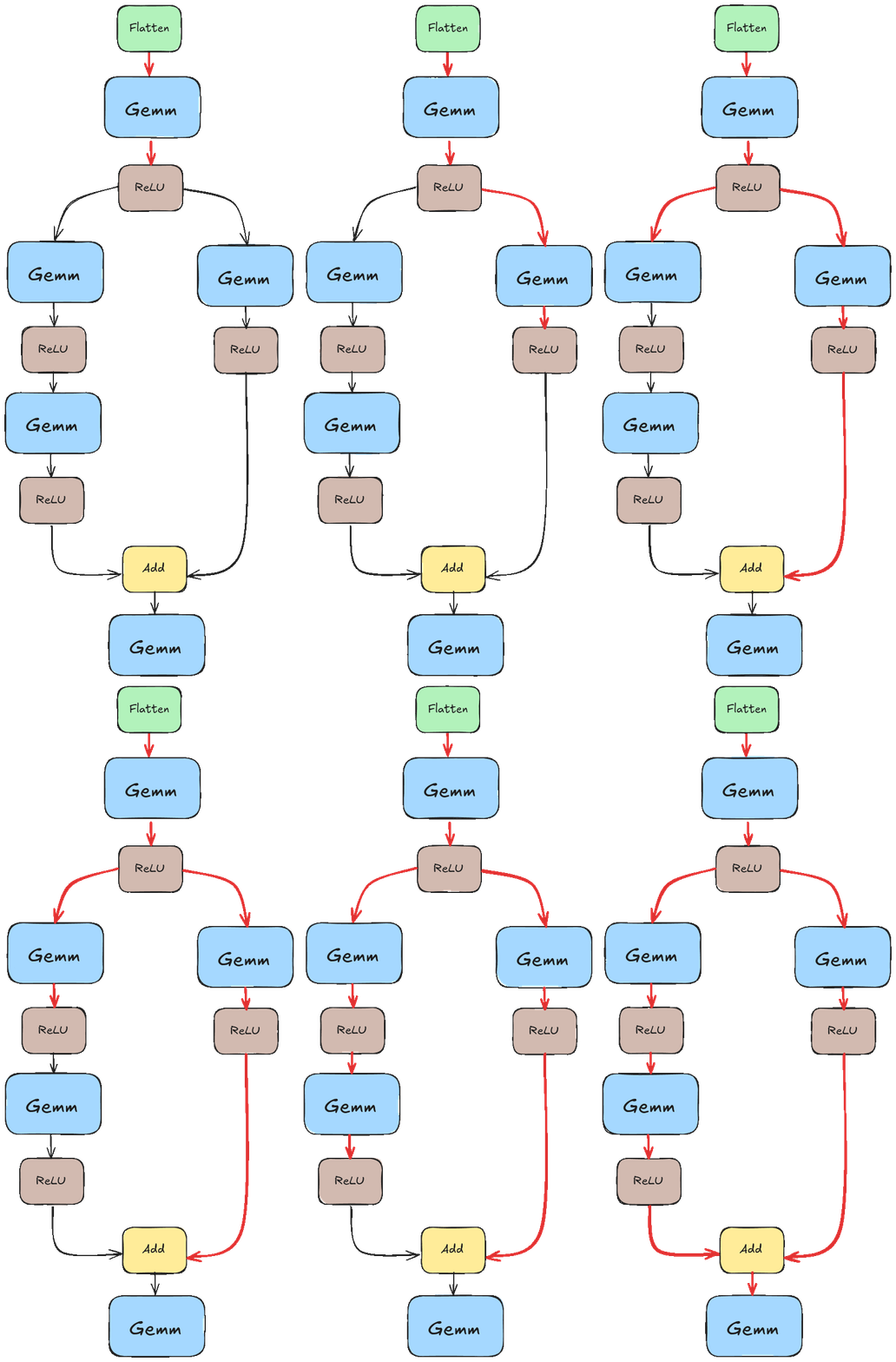
I’ll assume that our graphs are non-cyclic, i.e. we are dealing with DAGs. Still, we need to be careful to execute nodes in such an order that all intermediate results are ready when the node is executed.

If we didn’t pay special attention to this, we would likely run into a scenario like the one illustrated in the animation below. There we tried to execute “Add” before the results of the left branch were ready.

Trying to execute “Add” before the output of left ReLU is ready.

Instead, we want something closer to this.

Executing the model in topological order.

If you are already thinking if we could execute those two branches in parallel, then you are on the right track! We won’t go into that in this post as I haven’t implemented that logic yet, but it’s something I’d like to explore down the line.

So how do we get this order? We can use trusty topological sort which can be concisely implemented with depth-first search. Since we assume the model is static, it’s sufficient to compute the order once when the model first loads.

For those interested in seeing this implemented, you can read it here.

Inference

We’ve loaded the model, extracted its weights, constructed a graph, and sorted the graph’s node. We are all set for inference. I’ll skip input loading as it’s not particularly interesting. For our MNIST example, every input is a Tensor<uint8>(28, 28) representing a black-and-white image.

The infer() call iterates over topologically sorted nodes, for each node, it does the following:

Read input names used by the node.
Read inputs from a Tensor store into a vector of inputs.
Based on the node’s operation type, read additional input information, things as whether a matrix is transposed in Gemm.
Pass inputs to a corresponding operator function.
Save output to Tensor store or print if it’s the final result.

Here’s part of the method to get the main idea. You can see the full source code on github. Each case simply prepares inputs and passes them to the operator function.

The operator functions are implemented in operators.cpp. Since I decided to only support 4 operations, it’s not too bad to implement them from scratch. We are giving up some performance here, but I’d like to explore C++ profiling tooling in a follow-up post anyway. Especially around things like memory access and cache locality.

And that’s pretty much it. Let’s run the inference engine on this image of number 7.

michal@michal-lg:~/code/inference_engine$ /home/michal/code/inference_engine/build/src/engine_exe /home/michal/code/inference_engine/models/mnist_ffn_complex.onnx /home/michal/code/inference_engine/inputs/image_0.ubyte
Out: Tensor((1, 10)[[407.129, -1327.89, 827.717, 1137.59, -1497.12, -73.3868, -2284.66, 2266.74, 1.9645, 475.585]])

To determine the model’s prediction, we take the argmax of the output. Here the 7th (0 indexed) output is the largest, so the model correctly predicts the image is a 7!

Not bad for ~2000 lines of C++.

Thanks for reading! We’ve covered how inference engines work. Now that we have a minimal engine, I want to extend it. Let me know in the comments which improvements you’d like to see!

I hope you enjoyed this deep dive into inference engines! If you did, consider subscribing and/or following me on LinkedIn.

You might also enjoy some of my other posts. Maybe my deep dive into SQLite storage format or implementation of MapReduce from scratch?

From Scratch