
Optimizing matrix multiplication
Discovering optimizations one at a time

This article is all about performance optimizations - squeezing as much performance out of my CPU as I can.
I’ll start with a naive matrix multiplication in C and then iteratively improve it until my implementation approaches that of AMD’s bli_dgemm. My goal is not just to present optimizations, but rather for you to discover them with me.
As we go through this, we’ll learn a thing or two about compilers, assembly, and underlying hardware.
For the sake of ever finishing this article, I’ll focus purely on single threaded optimizations and will tackle parallelization in the future.
Setup
I’m running a Ryzen 5600H processor with 6 cores and12 threads. Each core has 32 KiB of L1d and L1i cache and 512 KiB of L2 cache. All cores share 16 MiB of L3 cache.
I’ll be using clang 18.1.3 on Ubuntu 24.04 throughout this article.
Matrix multiplication review
Given two matrices, A of n rows and k columns ((n,k) from now on) and a (k,m) matrix B of, the product of AB is an (n,m) matrix C. The element C[r][c] is defined as a the dot product of row r of A with the column c of B.
In summation notation:
Let’s use the mathematical definition as the starting point.
Naive implementation
The naive implementation is a direct translation of the mathematical definition to C. For simplicity’s sake, I’ll assume that matrices are square and their size is a power of 2.
Take a look to see if you spot anything surprising.

The restrict keyword tells the compiler that no other pointer will access the object, which in turn can allow the compiler to generate more optimized code.
Let me explain what column-major order is.
Storing matrices in memory
Column-major order is a flat representation of a matrix in memory such that columns are laid out sequentially. This approach is used by Fortran and many BLAS libraries, including AMD’s BLI.
The default ordering of 2D arrays in C/C++ is row major.

Measuring performance
I’ll be measuring the time required to multiply two 4096x4096 matrices of doubles.
I’ve chosen large matrices since some optimization are more pronounced when the matrices don’t fully fit in cache. With N=4096, the 3 matrices have a total size of (3*4096*4096*8)/(1024*1024) = 384 MiB, well over my 16 MiB L3 cache.
I also want to briefly discuss how I’ll compile code. Two main options are:
Introduce compiler flags as I introduce code optimizations
Enable all relevant optimization flags from the outset
I’ll go with the second option as I think it’s slightly more transparent. I’ll make sure to highlight when a code change causes “unintentional” optimizations. Unless stated otherwise, I’ll be using the following flags.
clang main.c matmul.c -std=gnu11 -O3 -DNDEBUG -march=native -mfma -ffast-math -mavx2 -lrt -lblis -o matmulBaselines
With code compiled, we can finally get first results.
The naive implementation multiplies two 4096x4096 matrices in leisurely 480 seconds,
michal@michal-lg:~/code/cpu_matmul$ ./matmul 4096
Elapsed execution time: 480.609548 sec; N: 4096, __TYPE__: double
while the much snappier bli_dgemm does it in 2.6s, around ~200x faster.
michal@michal-lg:~/code/cpu_matmul$ ./matmul 4096
Elapsed execution time: 2.564394 sec; N: 4096, __TYPE__: doubleSearching for bottlenecks
I’ve run the naive implementation through perf to collect performance counters. I’m using N=1024 matrices to speed things up when profiling.

The cache miss rate stands out to me as surprisingly large. Let’s use a little tool I wrote to better visualize memory accesses.
The video below shows both the logical and memory representations of matrices. As I step through the naive multiplication, notice where the accessed elements are located in memory.
Focus on which element of A gets accessed on each iteration. While in the logical representation we are accessing sequential elements within a row, due to the column-major order, these elements are actually N elements apart in memory. This is illustrated by the memory views at the bottom.
This is a major issue for sufficiently large matrices. Each access requries reading a new cache line from main memory. By the time the loop wraps around to the first element, chances are the original cache line was already evicted - forcing us to refetch it again.
I’ve illustrated a few iterations for matrix A. For illustrative purposes, I’m assuming a very small, fully associative cache that can only store 3 lines. Each cache line is 16 bytes or 2 doubles.
In the first loop, A[0][0] is read, it’s not in the cache, which results in cache miss, so the cache line has to be fetched from main memory. Notice that we fetch a full cache line even when we want only one element from it. On modern CPUs cache lines are commonly 64 bytes.
Next loop A[0][1] is read - again a cache miss.
Shame we didn’t read A[1][0] instead that we already fetched last iteration…
This keeps repeating until we loop back to A[0][0], but unfortunately, by that point, the cache line that contained A[0][0] was already evicted.

Try to convince yourself that if we instead iterated over matrix A in column order, the cache hit rate would significantly improve.
Loop reordering
Previously, we looped over the matrices in r, c, k order. Based on the findings in the last section, we’d like to iterate in row-order in the inner loop as much as possible.
We can just reorder these loops however we want without affecting correctness.

This presents us with two compelling loop orders: c, k, r and k, c, r.
I expect c, k, r to perform better since k is used as the row index in B, but intuition is often misleading, so let’s measure.
c, k, r:
michal@michal-lg:~/code/cpu_matmul$ ./matmul 4096
Elapsed execution time: 20.784827 sec; N: 4096, __TYPE__: doublek, c, r:
michal@michal-lg:~/code/cpu_matmul$ ./matmul 4096
Elapsed execution time: 51.014005 sec; N: 4096, __TYPE__: double
Just changing the loop order improved performance by ~20x.
Re-running perf stat shows a ~50x reduction in L3 cache misses.

Besides better access pattern, reordering loops allowed the compiler to vectorize some operations! Let’s discuss that next.
Inspecting Assembly
In this section we’ll look at how the assembly generated changes with vectorization on and off.
Non-vectorized
The figure below shows assembly for the inner loop with vectorization disabled. You can see the full function at compiler explorer.
Note: Here I only use compiler flags “-O3 -fno-vectorize”
I’ve annotated the interesting lines. Hopefully with some eye squirming you can convince yourself that the C code does logically translate into the assembly code on the right.
I grew up reading left to right so I prefer the AT&T assembly syntax. Sorry my Arab friends.

As highlighted, clang applied a loop unrolling optimization with a factor of 2, i.e. on each inner loop iteration, it calculates C[r][c] and C[r+1][c].
If it didn’t do this, 3 out of 7 instructions per inner loop execution would be purely for the loop overhead: increment counter, compare with loop limit, and jump. That would be expensive so unrolling ammortizes the cost. In fact, when the number of loop iterations is known at compile time, it’s very common to see completely unrolled loops.
Note how the compiler still generated LBB0_5 in case the loop has an odd number of iterations.
Vectorized

Modern CPUs have extra hardware to support SIMD (single instruction, multiple data) instructions. This lets a single CPU instruction operate on multiple registers in parallel.
I’m using the following compiler flags “-03 -ffast-math -mavx2” so that the compiler generates vectorized code. Again, feel free to play with the compiler explorer code.
I added a promise to the compiler that the data will be aligned to 32 bytes in memory. Some vectorized instructions require memory alignment or have a faster aligned variant.
I’ve again annotated the assembly.

The general sequence is very similar to before, but now the compiler uses AVX2 SIMD instructions. Availability of instructions depends on your CPU. You can read /proc/cpuinfo or run cpuid to see what your CPU supports.
Each AVX2 register (ymm) can fit 256 bits, i.e. four doubles, so each vmulpd, vaddpd, and vmovupd processes 4 multiplications, additions, and stores in parallel.
As you can see, the compiler again did some unrolling. This time with a factor of 4, so each inner loop execution produces 16 writes to C.
The following diagram illustrates the computational dependencies.

You can try to enable the fused add-multiply option on compiler explorer (-mfma flag) to see that
vmulpdandvaddpdinstructions get merged into a single one.
Given the 4x increase in parallelism, one would hope for 4x speedup - Unfortunately, I’m getting a more modest 1.5x improvement.
An important corollary of the AVX2 register size is that we can trade off numerical precision for higher parallelism. This extends to GPU-based ML training/inference, where half-precision fp16 or even fp8 floats are often used.
Just to briefly recap, we are currently sitting at ~10% of bli_dgemm’s single-threaded performance. Now might be a good time to make a second coffee and stretch a bit before proceeding.
Cache utilization
In this part we’ll cover a really cool optimization that’s unfortunately super unintuitive at first, at least to me anyways.
Let’s inspect the access pattern again. I encourage you to step through this yourself by selecting the naive order(jki) option in my matmul visualization tool.
Notice how the calculation scans through the entire matrix A N times? Ideally we’d load each element once, do all the computations where its needed, evict it, and never load it again.
Sticking with the 4x4 example; When A[0][0] is loaded, we only use it once to calculate the partical result C[0][0] += A[0][0] * B[0][0], before moving onto C[1][0] = A[1][0] * B[0][0].
Instead of moving onto A[1][0] immediately, we’d like to use A[0][0] in as many computations as we can. It’s also used as a dependency for C[0][1], C[0][2], and C[0][3].
But if we try to reorder computation to do that, we are somewhat back to a poor strided access pattern into C. Earlier we saw how strided access can cause elements to be evicted from cache before they are needed again when the full matrix doesn’t fit in cache. Well, what if we could make it fit into cache?
If we can restructure the product of two large matrices into products of smaller matrices, then we can tune the small matrix size so that things fit nicely in cache!
Tiling
The technique I long-windedly introduced above is known as tiling. Let’s first see tiling in action, then I’ll show you the code, and then we’ll do some benchmarking.
I’m using tile size (or block size) of 2 and yet again, you can play with it in the matrix visualization tool.
In the non-tiled version, we scanned through the entire matrix A N times. You can check that every element of A is still accessed exactly the same number of times as before. So what changed? Each tile only needs to be loaded once into cache, since we can tune it to fit.
In general, we are hoping to reduce the number of cache misses by a factor proportional to the tile size.
More loops
Below you can see the tiled implementation. It’s starting to get a bit ugly with the tiling loops, but try to read through it anyways. Note that we do exactly the same amount of work as before (minus look overhead), just in a different order that better utilizes the cache.

I selected the tile_size through the best technique known to man - trying a bunch of values and picking the best.
4 - 45s
8 - 16s
16 - 19s
32 - 10s
64 - 7.3s
128 - 6.6s
256 - 9s
We are finally getting to pretty small numbers where sub-second precision is starting to matter. However, there can be a decent run-to-run variance. This variance is primiarly caused by other processes on my system polluting CPU cache, process context switches etc.
For the different tile sizes above, I ran the measurement a few times for each setting and picked the minimum duration for each. This seems counterintuitive, but when noise is the main source of variance, the fastest run is the one with the least noise.
6.6 seconds is a ~3x improvement, putting us at ~30% of bli_dgemm performance.
Tile size analysis
Can we explain why the 128 x 128 tile size performs the best on my system?
When I measure the L3 and L2 cache misses for N=4096 matrices, it turns out that tiled_dgemm performs significantly worse on both counts than our previous implementation. L3 misses are at ~2B compared to ~500M for naive_ordered_dgemm.
The number of L3 reads is lower by about 10B, but I’m not super positive that fully explains the better performance. Suffice to say I was pretty confused at this point. Inspecting the newly generated assembly shows very aggressive unrolling in the tiling block. My best guess is that despite the large cache miss count, the CPU is able to hide read latencies by overlaying reads and computation thanks to the aggressive unrolling.
Still, the fact that number of cache misses went up is surprising to me. Let’s explore that next.
Cache hardware
Until now we were assuming a fully associative cache - one where a cache line can be stored anywhere. Being able to store a cache line anywhere sounds convenient, but the flip side is that to check if a given cache line is stored, all entries need to be checked.
Instead, caches are commonly partitioned into sets of k cache lines. Then for a cache line, based on its address, its sufficient to search through the k lines in its corresponding set.
Let’s see how given an address, we determine where in cache it can reside. I’m basing this on my L3 cache specs: k=16-way associative cache, B=64 byte cache line, M=16 MiB cache size, and w=64 bit words.
Address resolves to a cache line using the following mapping:
offset - lg(B=64) = least significant 6 bits
set - lg(M/kB) = lg(16MiB/(16*64)) = 14 bits
tag - 64 - 14 - 6 = 44 bits

Note that offset contains the least-significant bits. This intuitively makes sense - we want addresses in close proximity to belong to the same cache-line.
So, how does this relate to the increased L3 misses we saw earlier?
Let’s focus what happens when we load a single tile into memory. Suppose that tile[0][0] element is at address x. Then the element tile[1][0] is at address x+8, tile[2][0] at x+16, etc. 8 consecutive elements will belong to the same cache line. tile[8][0] will have address x+64, which flips the 7th bit, so it belongs to a different set. The last element of the first tile column will have address x+127*8 , which means that first column required ceil(127*8 / 64) = 16 lines in 16 different cache sets.
When we wrap around to the next column, tile[0][1] has address x+4096*8 or x+2^15. Recall that we are dealing with 4096 x 4096 matrices. In general, the address of tile[0][i] will be x + N*sizeof(double)*i, where N is the matrix dimension.
Notice how for my L3 cache, only the bottom 20 bits are used to map an address to the cache. When two addresses differ only in top 44 bits, those two address will map to the same cache set. Given the earlier formula, we can calculate which columns will start mapping to the same cache set by solving for i.
x + 2^20 = x + 4096*8*i → i = 2^20 - 2^15 = 2^5 = 32.
So we know that tile[0][0], tile[0][32], tile[0][64], and tile[0][96] all map to the same cache set. Below is a more dramatic visualization. Colored blocks within the tile depict cache lines that map to the same cache sets.

Is this really an issue? After all, we have 16 cache lines per set.
Well, that’s true, but we also have 2 other matrices and there are other processes running on my system. Creating unnecessary pressure on a given cache set increases likelihood of so-called conflict misses. This happens when a line is evicted because its cache set is full.
This issue would be even more pronounced in L2 and L1 caches that are smaller and typically have lower associativity.
Packing
If we lay out a 128 x 128 tile of doubles sequentially in memory, the difference between the first and last address is 2^8*2^8*2^3 = 2^19. With this we don’t run into the same cache set conflicts and the tile is uniformaly distributed across different cache sets.
This suggests an optimization strategy - copy tiles into arrays and do the tile-tile matrix multiplication over the arrays. Our hope is that the better cache hit rate will compensate for the extra copying work.
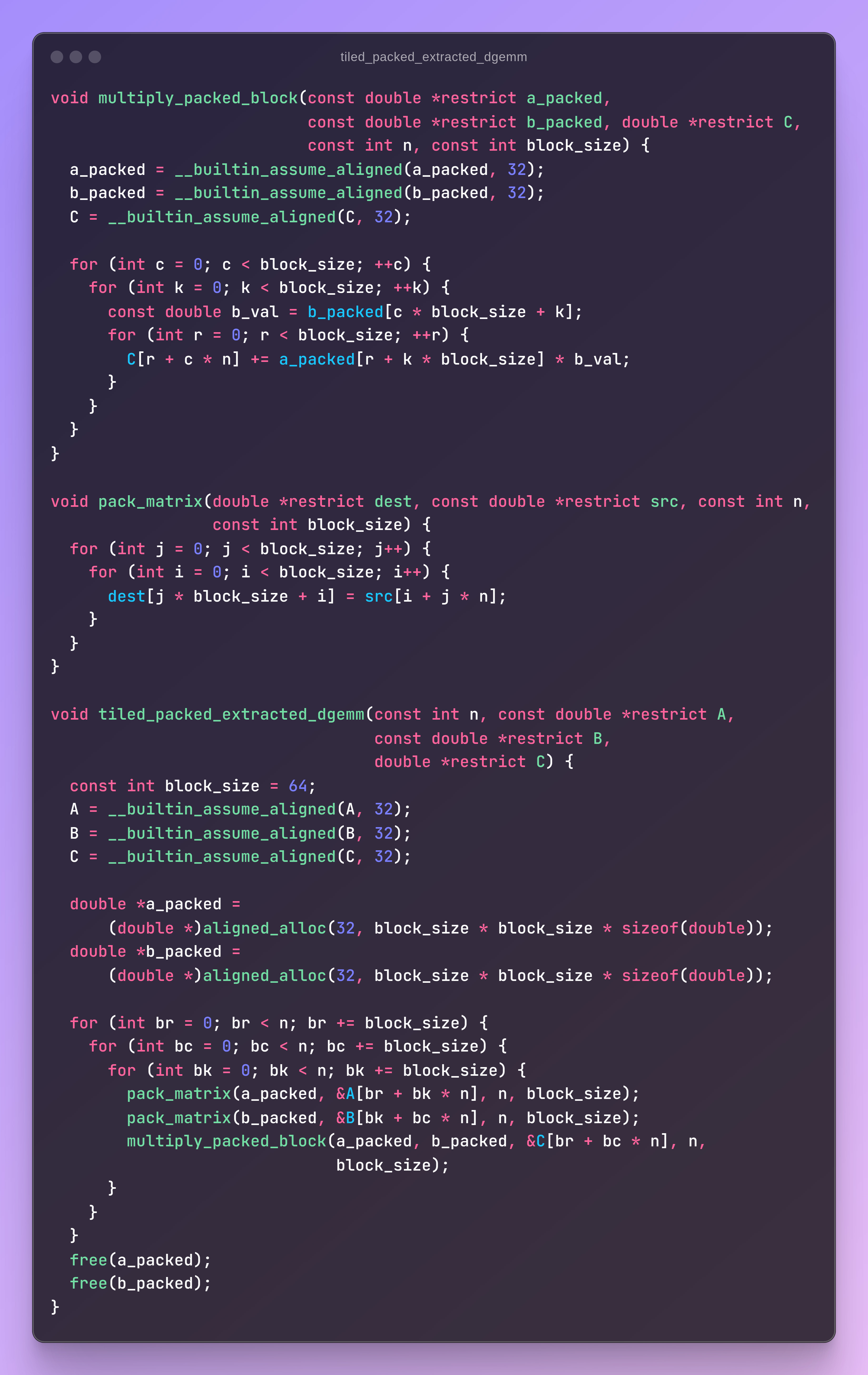
Instead of directly operating on matrices, we now copy tile of A and tile of B into helper arrays and operate on those. You can see the code and generated assembly at compiler explorer. I reran experiments for different tile sizes and 64 happens to be the optimal size.
I also extracted the inner loops into a separate function, which appears to help the compiler generate more optimized assembly on my hardware. I suspect this has to do with better register allocation. The extraction alone improves runtime from the previous ~6.6s to ~6.2s. Note that the function gets inlined so there’s no call overhead.
So how much does this improve performance?
*drum roll*
We are down to ~4.4s or around 60% of bli_dgemm. Relative to the naive implementation, the current solution is over 100x faster.
As a final sanity check, L3 cache misses did go down by about 4x.
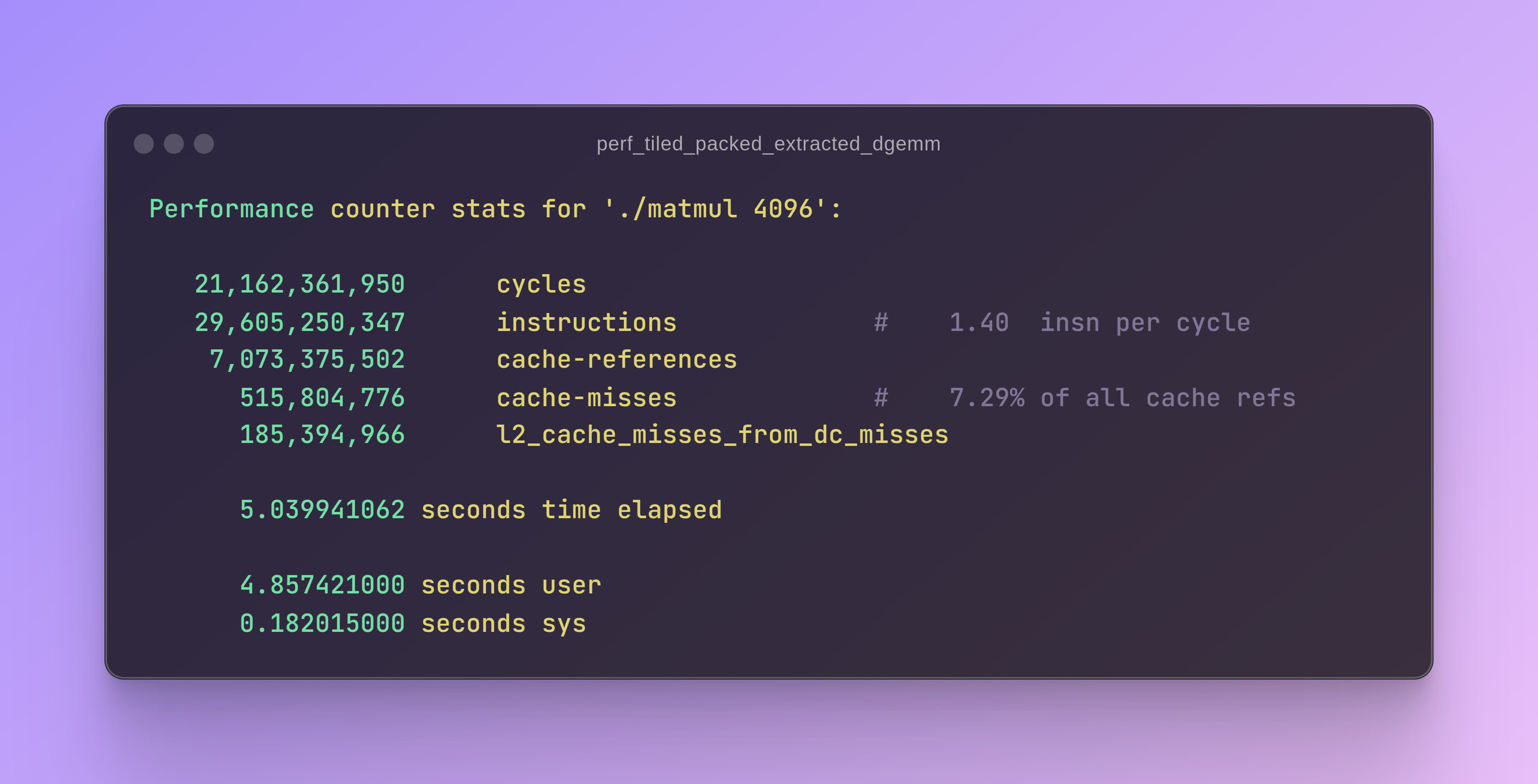
bli_dgemm still runs circles around my implementation when it comes to L2 cache misses and instructions per cycle. That being said, I’m happy with getting within 2x of bli_dgemm.
The comparison isn’t completely fair. bli_dgemm supports arbitrary matrix sizes, while I’m only focusing on large, square, power-of-two sized matrices. If I supported arbitrary matrix sizes, I’d need to add extra instructions for boundary checks.

Next steps?
There are many optimizations we haven’t attempted yet. For instance, we could add another level of tiling for L2 cache and even for L1 cache. We could also experiment with directly using compiler instrinsics for SIMD instructions. Memory prefetching instructions are also worth experimenting with. There are also recursive algorithms that split matrices into smaller ones instead of using tiling.
While exciting, this article has gotten a lot longer than I expected, so I’ll leave those optimization for a potential followup article.
If you this domain interesting and would like to learn more, I recommend these resources:
MIT’s 6.172 on OCW - a fantastic introduction to performance engineering. I’ve been auditing it while writing this article.
Simon’s matrix multiplication article - Simon is a performance engineer at Anthropic. His article covers most of the optimizations I covered here. I like Simon’s succint style and gorgeous illustrations.
OpenBLAS repository on github - highly optimized open-source kernels.
I hope I conveyed not just what optimizations exist but also how one might go about discovering them. I find the latter a lot more satisfying.
If you enjoyed this article, consider subscribing. I’m also somewhat active on LinkedIn, so consider connecting with me there.
After a well-deserved break for reading this far, perhaps check out some of my other articles.
Linux container from scratch

I recently built a docker clone from scratch in Go. This made me wonder - how hard would it be to do the same step-by-step in a terminal? Let’s find out!
GPU Programming

One of the great joys of software engineering is dispelling magic. I’ve written code that executed on a GPU using frameworks like PyTorch or TensorFlow, but I never understood the “how”. It’s time to dispel the magic of GPU programming and learn how it works under the hood.
How does SQLite store data?

Recently I’ve been implementing a subset of SQLite (the world’s most used database, btw) from scratch in Go. I’ll share what I’ve learned about how SQLite stores data on disk which will help us understand key database concepts. Thanks for reading Michal’s Substack! Subscribe for free to receive new posts and support my work.